Trading Book
Correction — 22 September 2026: The original post overstated what this experiment showed. The linked notebook trains and evaluates on the same period, and the implemented learner uses bagged randomized trees, not Q-learning. I’ve corrected the method and cost settings below. The chart is retained from the original post; the experiment has not been rerun for this revision.
Why I built it
I spent two days building an algorithmic trading starter notebook. At work we were taking a different approach to an FX trading project, and I wanted an alternative starting point that we could compare with it. The techniques came from Georgia Tech’s Machine Learning for Trading, taught by Tucker Balch when I took it.
I also committed the data to the repo to make the example easier to follow. Not my finest engineering practice, but it made sharing the experiment straightforward.
From prices to positions
Our internal project used an LSTM. For this notebook, I put historical price information into technical indicators so that each day became a row of features. That made it possible to use a tree-based learner without feeding it an entire sequence.
The question to test
Can these indicators help predict future returns well enough to improve on a benchmark after costs, on dates the learner has not seen? That is the hypothesis this project would need to test.
The original post jumped from that possibility to rejecting the Efficient Market Hypothesis. That was too broad. Since the inputs come from historical prices, the relevant comparison is with weak-form efficiency, which concerns information in past prices and trading volume. The CFA overview of market efficiency distinguishes this from the semi-strong and strong forms. This notebook does not establish a rejection of any of them.
What the code implements
The historical StrategyLearner uses bagged randomized trees. The selected inputs are upper_band, lower_band, and RSI. Training labels come from subsequent returns and indicate a target position: short, cash, or long. This is supervised learning. Q-learning appears as an alternative in the code, but its constructor is commented out.
A position is different from an order. The strategy converts changes in target position into trades. Moving from cash to 1,000 shares long requires buying 1,000 shares. Moving from 1,000 shares long to 1,000 shares short requires selling 2,000. Keeping the same position requires no trade.
The output is an orders file containing dates, symbols, buy/sell directions, and share counts. Calling it an “order book,” as I did originally, was misleading.
What the demonstration shows
The historical notebook compares the learned strategy with a manual strategy and a benchmark. It trains on JPM data from 2008–2009 and calls testPolicy on that same period. It defines a 2010–2011 period, but does not use it in the displayed evaluation.
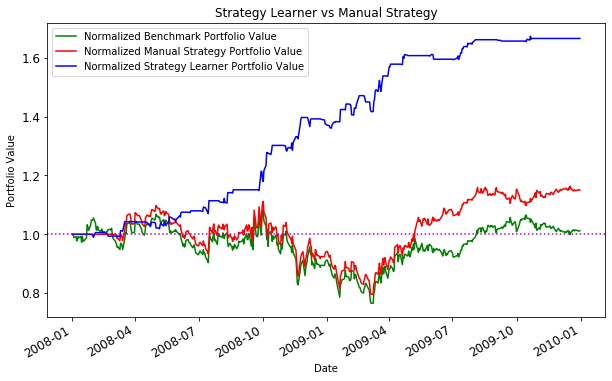 Original chart from the 2020 post. The linked notebook evaluates on the training period; this result has not been reproduced for the September 2026 correction.
The learned strategy’s curve looks encouraging, but an in-sample comparison cannot show how it would perform on unseen dates. The notebook uses zero transaction commission and an impact parameter of 0.005 for the learned and manual strategies. There is a cost assumption in the simulation; it is still a simplified one.
Backtesting still needs work
The observed limitation is the reuse of the training period for evaluation. A next test would need a later, untouched period, with all model choices made beforehand and training labels kept from crossing the split boundary.
Execution timing and leakage also need an audit: were the indicators available before the assumed trade, and did any preparation step use future information? Costs would need to cover realistic execution, including spreads, slippage, and short-borrow costs where relevant. Stock selection can introduce survivorship bias, and repeatedly trying strategies on the same period can turn it into another tuning set. These are issues to check, not findings from a completed audit of this repo.
For now, the notebook demonstrates the path from indicators to positions, orders, and simulated portfolio values. It does not demonstrate live profitability.
The setup I used in 2020
AWS setup
At the time, my preferred setup was an AWS Deep Learning AMI. I suggested a p2.xlarge instance and the Fast.ai AWS setup notes. Those were 2020 recommendations, not a current hardware or pricing guide.
Alternative setup
I also used Google Colab for experiments, with data loaded through Google Drive. That was a convenient alternative for me then. The old setup instructions should be treated as historical too.
Ideas I had for the next version
My original list included deep reinforcement learning, LightGBM with more data, stacking, news data, and an entry in Two Sigma’s financial-news Kaggle competition. These were ideas, not completed work.
Before extending the model list, the experiment needs a chronological out-of-sample evaluation. That is the missing comparison in this two-day starter project.